rudro.dev
Tue Sep 05 2023

Harmonic Motion Analyzer
GitHub - https://github.com/rudrodip/Harmonic-Oscillator-CVTwitter - https://x.com/rds_agi/status/1721512171354615870Website - https://www.rudrodip.tech/blog/harmonic-oscillation-analyzerYoutube - https://www.youtube.com/watch?v=dalsCsHtreU&t=1220sLinkedIn - https://www.linkedin.com/posts/rudrodip_creative-coding-competition-results-activity-7127276230269161472-mjKp
Python
OpenCV
SciPy
PyQT5
PyQT5-graph
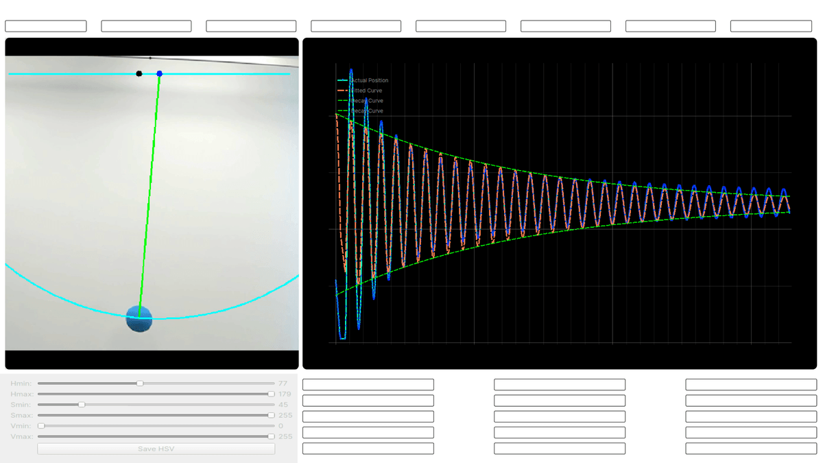
Harmonic Motion Analyzer is designed to analyze the harmonic oscillation of an object using computer vision techniques, it can analyze live video feed, and has nearly 99.86% accuracy.
Overview of the project
This project is a powerful tool designed to analyze harmonic oscillation of objects using computer vision techniques. Leveraging a variety of libraries, including OpenCV for video feed processing, SciPy for data analysis, NumPy for numerical operations, and PyQt5 for a user-friendly graphical interface, it offers a wide range of features to facilitate detailed analysis.
This project was submitted for the Creative Coding Competition organized by Radu Mariescu-Istodor. I actually scored the highest in the competition (46/50), here's the video reviewing my project by Radu Mariescu-Istodor
Key Features
-
Bob Color Detection: The system can accurately detect the bob of any color, providing flexibility in object selection.
-
Contour Detection Options: Choose from three contour detection methods - color-based, edge-based, or circle detection - to suit your specific tracking needs.
-
Video Source Flexibility: Analyze harmonic oscillations from various sources, including:
- Local Video: Process videos stored on your device for in-depth analysis.
- Webcam: Utilize your webcam for real-time tracking and motion analysis.
-
Display Options:
- Main Video: Observe the original video feed.
- Contours: Visualize the detected contours for better tracking insights.
- Mask: Monitor the real-time masking process and make adjustments as needed.
-
Real-time Parameter Adjustment: Easily fine-tune masking parameters in real time and save your configurations for future reference.
-
Parameter Saving: After prediction, you can conveniently save the calculated parameters for further analysis and documentation.
-
Frame Offset Control: Within the code, set a frame offset and utilize a built-in function to save critical data points, streamlining the analysis process.
-
Rotation Compensation: The system intelligently compensates for video rotation, ensuring accurate analysis even when dealing with rotated footage.
-
Prediction Capabilities:
- Pivot Point Prediction: Accurately predict the pivot point of the bob's motion.
- Mean Point Determination: Find the mean point of the bob's trajectory.
- Path Analysis: Analyze the bob's path and generate predictions of its corresponding harmonic motion equation.
-
Physical Properties Estimation: Utilizing parameters derived from the predicted harmonic motion equation, the system can estimate crucial physical properties of the system, such as the length of the string or other relevant characteristics.
This project provides a robust and versatile platform for in-depth analysis of harmonic oscillations using computer vision techniques. Its user-friendly interface, real-time adjustments, and predictive capabilities make it an invaluable tool for researchers, educators, and enthusiasts exploring dynamic systems and motion analysis.
How to use it?
It is highly advisable for you, to thoroughly go through UI section. Doing so will greatly facilitate the project setup process and enable a better grasp of the user interface (UI). Your understanding of this section is pivotal in ensuring the efficient configuration of the project and in comprehending the UI.
Prerequisites
Before you begin, ensure you have met the following requirements:
- Python 3.6 or higher installed on your system. You can download Python from python.org.
- Git installed (optional, but recommended for cloning the repository).
Setting Up a Virtual Environment
It's a good practice to work within a virtual environment to isolate your project's dependencies. Here's how to set up and activate a virtual environment:
-
Open a terminal or command prompt.
-
Clone this repository to your local machine:
git clone https://github.com/rudrodip/Harmonic-Oscillator-CV- Navigate to your project directory:
cd Harmonic-Oscillator-CV- Create a virtual environment (replace
venvwith your preferred name):
python -m venv venv- Activate the virtual environment:
- On Windows:
venv\Scripts\activate- On macOS and Linux:
source venv/bin/activate- Your terminal prompt should now show the name of the virtual environment, indicating that it's active.
Installing Dependencies
Once you have your virtual environment set up and activated, you can install the project's dependencies:
-
Make sure you are in your project directory with the activated virtual environment.
-
Install the dependencies from the
requirements.txtfile:
pip install -r requirements.txtUsage
- Run the main application script:
python app/app.pyIf you find any difficulties installing or running it, feel free to contact me. I have developed this project on linux (ubuntu 22.04), if you have any issues installing packages on your machine, feel free to change the code.
Note: The OpenCV library you will be using for this project is opencv-python-headless (not opencv-python), so make sure you have the correct library installed in virtual environment, otherwise uninstall opencv-python and reinstall opencv-python-headless using this command
pip install opencv-python-headless --no-cache-dirUser Interface
Let's take a closer look at the user interface (UI) of this project, which plays a central role in interacting with the video processing and analysis. The UI design is straightforward and user-friendly, consisting of several key elements:
Buttons and Dropdowns

- Run: Initiates video processing after selecting a video source (file, webcam, or URL).
- Stop: Halts the video processing and output.
- Select Video: Allows the user to choose a video file for analysis.
- Webcam: Selects the webcam as the video source.
- URL: Enables video processing from a provided URL.
- Hide Params: Toggles the display of parameters such as pivot point, circular path, and the string connecting the pivot and the bob.
Dropdowns:
-
Display Options: Allows you to select how the video is displayed. Options include "Image Contours" (showing the detected bob with a bounding box), "Main Video" (the raw video), and "Mask" (the mask used for detecting the bob).
-
Color Detection: Provides options for how the image processor detects the bob. Options include "Color detection using HSV range" (recommended), "Edge detection," and "Circle detection."
HSV Range Sliders

These sliders are used for color detection. By adjusting the sliders, you can define the HSV (Hue, Saturation, Value) color range used by the image processor to detect the object. You can save these settings by clicking the Save HSV button.
A recommended workflow is to set the display option to "Mask," select "Color Detection," run the video, and fine-tune the sliders until you achieve optimal object detection.
Analyze Widget

The analyze widget is a crucial part of the UI. After selecting a video source and running the analysis, you can click the Estimate button. This action triggers the fitting of a curve to the data points collected by the image processor. The widget provides parameters and settings for this analysis. You can also save these parameters using the Save button.
Graph

The graph section is perhaps the most visually appealing part of the UI. It utilizes the pyqtgraph library and offers advanced graph manipulation capabilities. You can scale, zoom, pan, and save the graph in various formats (SVG, PNG, Matplotlib window, CSV). Its flexibility and interactive features make it a powerful tool for visualizing and analyzing the harmonic oscillation data.
Project Sections
The project can be divided into three major sections:
-
Programming: In this section, I've covered the development of the user interface and the image processing pipeline, using libraries such as OpenCV and
cvzone. The UI creation was straightforward, thanks to Python and PyQt5. -
Mathematics: In the mathematics section of the project, I utilize powerful mathematical tools to extract insights from the data
-
Curve Fitting with
curve_fit: I use SciPy'scurve_fitfunction to fit collected data points to a damped oscillation function. This helps me accurately detect and analyze harmonic motion patterns. -
least_squarefor Circular Path Detection: Theleast_squarealgorithm is not only used for curve fitting but also for assessing the accuracy of circular paths. It ensures that predicted paths closely match the actual object motion, validating the precision of path predictions and harmonic motion analysis.
-
-
Physics: While closely related to mathematics, the physics aspect primarily focuses on extracting physical parameters such as pendulum length and pivot point location. These parameters provide valuable insights into the object's harmonic motion.
This breakdown of the user interface and project sections should provide a clearer picture of the project's structure and functionality.
Programming
Let's dive deep 🙂
User Interface (UI)
Creating the user interface for this project was a relatively smooth process. Thanks to Python and PyQt5, I was able to design the interface without much hassle. While the UI design took some effort due to its complexity, it wasn't the most challenging part of the project.
Image Processing
- magic 🪄
OpenCV and cvzone
Image processing is where the real magic happens in this project. OpenCV is a fantastic library, and it played a central role in handling the video feed. It allowed me to perform tasks like object detection, tracking, and image manipulation with ease.
Additionally, I leveraged cvzone for contour detection, which was particularly helpful for identifying objects based on their HSV color range. This library simplified a crucial part of the image processing pipeline.
Main Loop Workflow
The main loop of the project was the heart of the image processing section. Here's how it worked:
-
Frame Acquisition: At the beginning of each iteration, I obtained a new frame from the video feed.
-
Contour Detection: With the help of
cvzone, I detected contours in the frame. This step was crucial for pinpointing the object of interest, often based on its distinct color range in the HSV color space. -
Pivot Point Estimation and Path Prediction: This step was the real technical challenge. I used the
least_squarealgorithm from SciPy to estimate the pivot point of the oscillating object. Moreover, I employed this algorithm to predict the future path of the object. This was essential for analyzing the object's harmonic oscillation characteristics, which I'll elaborate on in the mathematics section. -
Data Transfer to UI: To keep the user informed, I sent relevant data, including the transformed position (
transformed_x) and frame count (frame_count), back to the main user interface. -
Frame Rendering: The current frame was also sent to the UI for real-time rendering, allowing users to visualize the object's motion and the ongoing analysis.
-
Repeat: These steps were executed in a continuous loop for every frame in the video feed, enabling the real-time analysis of the object's oscillations.
Mathematics
In this section, I'll take you on a mathematical journey through the key tools and techniques that drive this project, making it easier to understand.
Detecting Circular Motion with least_square
In this section, I'll walk you through the critical steps involved in using least_square to detect circular motion, even if the video is rotated. Let's dive into how I achieved this:
1. Contour Extraction
Why? To accurately detect the position of the oscillating object (the bob) in each frame.
How? I started by extracting the object's contours from each frame of the video feed. Contours are like outlines that provide precise coordinates of the object's location.
2. Calculating Residuals
Why? To assess how closely the detected path resembles a circle and understand any deviations.
How? I implemented the circle_residuals function, powered by least_square. This function calculates the differences between the observed data points and the expected points on a circle.
def circle_residuals(params, x, y):
  """
  Calculate the residuals for circle fitting.

  Args:
      params: Parameters of the circle (a, b, r).
      x: x-coordinates of data points.
      y: y-coordinates of data points.

  Returns:
      Residuals indicating the difference between the data points and the circle model.
  """
  a, b, r = params
return np.sqrt((x - a) ** 2 + (y - b) ** 2) - rWhere:
- represents the predicted residuals.
- is the radius of the circle.
- and are the arrays containing the x and y coordinates of data points.
This equation calculates the residuals for fitting a circle to a set of data points.
3. Optimization
Why? To fine-tune and optimize the parameters of the rotated circle for accuracy.
How? I let least_square do its magic. It optimized the circle's parameters, including center, radius, and rotation angle. This step ensures that the predicted circular path aligns closely with the actual object path, even if there is rotation in the video.
The Result? A robust method for accurately detecting circular motion, even if the video is rotated. It's like having a compass that guides us to the truth in a sea of data.
4. Pivot Point and Rotation
Why? To account for video rotation and accurately transform the object's coordinates.
How? When I identified the circular motion, I used a straightforward method. First, I calculated the average position of the pendulum. Then, I found the tangent between the pivot point and this mean position. This allowed me to determine the precise angle of rotation, which, in turn, enabled me to accurately adjust the bob's x and y coordinates.
The Result? This entire workflow ensured that I could analyze harmonic motion, correct for video rotation, and extract precise data for further analysis.
Fitting the Harmonic Puzzle with curve_fit
At the heart of this mathematical marvel lies the curve_fit function from SciPy. This is where the magic unfolds, as I delve deep into the data to uncover the secrets of harmonic oscillations.
Why ?
Purpose: curve_fit serves as my mathematical detective, deciphering the hidden patterns within my data. Its mission? To find the perfect mathematical equation that describes the object's motion.
How it Works:
-
Collect Data: I start by collecting data points that represent the object's position over time. These data points are like breadcrumbs left by the oscillating object.
-
Select a Model: I choose a model that I believe fits the data. In my case, it's a under damped oscillation function. This function includes parameters such as amplitude, omega, damping coefficient, and phase, which describe the expected motion of the object.
Equation for the under-damped oscillation function
def underdamped_harmonic_oscillator(t, A, gamma, w, phi, C):
    """
    Calculate the position of an underdamped harmonic oscillator at time t.

    Args:
        t: Time values.
        A: Amplitude of oscillation.
        gamma: Damping coefficient.
        f: Frequency of oscillation.
        phi: Phase angle.
        C: Constant offset.

    Returns:
        Position values at the given time points.
    """
return A * np.exp(-gamma * t) * np.cos(w * t + phi) + C-
Let
curve_fitWork Its Magic: This is where the excitement builds. I feed the data points and my chosen function (the damped oscillation model) intocurve_fit. This function employs a clever optimization algorithm to adjust the model's parameters until it best matches the data. -
Parameter Extraction: After the optimization done, I extract the best-fit parameters. These parameters are like the missing pieces of my puzzle, allowing me to quantify the motion's amplitude, omega, damping coefficient, and phase.
x_data = data[:, 0]
y_data = data[:, 1]

params, _ = curve_fit(
    underdamped_harmonic_oscillator,
    x_data,
    y_data,
    p0=initial_guess,
    bounds=(lower_bounds, upper_bounds),
    maxfev=2500,
    ftol=1e-6,
)

# Extract the fitted parameters
A, gamma, w, phi, C = params
The Result? A beautifully fitted curve that elegantly captures the essence of harmonic motion. It's akin to assembling a puzzle and revealing the complete picture.
Physics
Now, let's explore the fascinating physics behind harmonic motion in a way that's easy to understand. Imagine we have a system—a mass attached to a spring with a damper—and it's doing some interesting things.
The Second-Order ODE: What's That?
In the realm of physics, we often describe the motion of objects using mathematical equations. In our system, we employ a second-order ordinary differential equation (ODE):
Here's the equation in its mathematical form:
Here's what each component means:
- is the object's position at time .
- is its velocity, and is its acceleration.
- is the object's mass.
- represents damping coefficient, which resists motion.
- is the spring constant, indicating how stiff the spring is.
This equation is essential for understanding our system's physics.
The Harmonic Solution: It's Beautiful
Now, here's the cool part. When conditions are right (meaning the damping isn't too strong), our system behaves in a super cool way. We can describe its motion with a beautiful equation:
Let me break it down:
- is the amplitude, which is like how far our mass swings.
- represents damping coefficient, which resists motion.
- is the angular frequency.
- is the phase angle.
- is just a constant that might shift our motion up or down.
Relating to a Damped Pendulum
You might wonder, how is this related to a damped pendulum? Well, it turns out, the equations are pretty similar! In the case of a damped pendulum, instead of a mass moving along a spring, we have a bob swinging on a string.
The equation for a damped pendulum looks like this:
- is the angle our pendulum makes with the vertical.
- represents damping coefficient, which resists motion.
- is the natural angular frequency of the pendulum, and it depends on the length of the string and gravity.
Why Matters
In both systems, the value of is super important! It tells us how fast things are moving or swinging. For a pendulum, it's linked to the length of the string. It's like the heartbeat of our system, determining how it behaves over time.
Measuring Pendulum String Length
Let's explore a clever method for measuring the length () of a pendulum string, taking into account the damped conditions of the pendulum's motion. This approach is not only ingenious but also practical, especially when dealing with complex pendulum systems.
Step 1: Analyzing Damped Harmonic Motion
Our first step involves carefully observing the pendulum's harmonic motion under damped conditions. We need to record essential data, with a keen focus on determining the angular frequency () that characterizes the pendulum's oscillation in the presence of damping.
Step 2: The Damped and Relationship
The angular frequency () for a damped pendulum system can be expressed in terms of the natural angular frequency () and the damping coefficient () as follows:
Where:
- is the angular frequency of the damped pendulum.
- is the natural angular frequency (undamped) of the pendulum, given by , where is the acceleration due to gravity and is the length of the pendulum.
- (gamma) is the damping coefficient, representing the strength of damping in the system.
This formula accounts for the effect of damping on the oscillatory motion of the pendulum. When is non-zero, it reduces the angular frequency from its undamped value , resulting in damped oscillations.
The formula for the natural angular frequency () of an undamped pendulum is given by:
Where:
- is the natural angular frequency of the undamped pendulum.
- is the acceleration due to gravity.
- is the length of the pendulum.
This equation tells us that the natural angular frequency () is inversely proportional to the square root of the length of the pendulum (). Therefore, longer pendulums have smaller natural angular frequencies, and shorter pendulums have larger natural angular frequencies.
Step 3: Determining
We can rearrange the equation to calculate the length of the pendulum string ():
Step 4: Handling Compound Pendulums
A compound pendulum, also known as a physical pendulum, is different from a simple pendulum because it has an extended mass distribution rather than a point mass at the end of a string. To calculate the angular frequency () for a compound pendulum, you need to consider the moment of inertia (MOI) of the pendulum about its pivot point.
The moment of inertia () depends on the shape and distribution of mass in the pendulum. The moment of inertia of the spherical bob about its center is given by:
Where:
- is the mass of the spherical bob.
- is the radius of the spherical bob.
The moment of inertia of the pendulum about its pivot point, taking into account both the bob and the string, is the sum of the moments of inertia of the bob and the string:
Where:
- is the moment of inertia of the compound pendulum about its pivot point.
- represents the moment of inertia of the string of length .
Now, you can use the formula for the natural frequency () of the compound pendulum:
Where:
- is the natural frequency of the compound pendulum.
- is the mass of the pendulum.
- is the acceleration due to gravity.
- is the distance between the pivot point and the center of mass of the pendulum.
- is the moment of inertia of the pendulum about the pivot point.
So, we can say (natural frequency of a damped pendulum) is a function of both length () and radius ().